JW Mason – Page 23 – J. W. Mason

Links for March 14

A few things elsewhere on the web, relevant to recent conversations here.

1. Michael Reich and his colleagues at the Berkeley Center for Labor Research have a new report out on the impacts of a $15 minimum wage in New York. It does something I wish all studies of the minimum wage and employment would do: It explicitly decomposes the employment impact into labor productivity, price, demand and labor share effects. Besides being useful for policy, this links nicely to the macro discussion of alternative Phillips curves.

2. I like Susan Schroeder’s idea of creating a public credit-rating agency. It’s always interesting how the need to deal with immediate crises and dysfunctions creates pressure to socialize various aspects of the financial system. The most dramatic recent example was back in the fall of 2008, when the Fed began lending directly to anyone who needed to roll over commercial paper; but you can think of lots of examples, including QE itself, which involves the central bank taking over part of banks’ core function of maturity transformation.

3. On the subject of big business’s tendency to socialize itself, I should have linked earlier to Noah Smith’s discussion of “new industrialism” (including my work for the Roosevelt Institute) as the next big thing in economic policy. Eric Ries’ proposal for creating a new, nontransferable form of stock ownership reminded me of this bit from Keynes: “The spectacle of modern investment markets has sometimes moved me towards the conclusion that the purchase of an investment [should be] permanent and indissoluble, like marriage, except by reason of death or other grave cause… For this would force the investor to direct his mind to the long-term prospects and to those only.”

4. In comments to my recent post on the balance of payments, Ramanan points to a post of his, making the same point, more clearly than I managed to. Also worth reading is the old BIS report he links to, which explicitly distinguishes between autonomous and accommodative financial flows. Kostas Kalaveras also had a very nice post on this topic a while ago, noting that in Europe TARGET2 balances function as a buffer allowing private financial flows and current account balances to move independently from each other.

5. I’m teaching intermediate macroeconomics here at John Jay, as I do most semesters, and I’ve put some new notes I’m using up on the teaching page of this website. It’s probably mostly of interest to people who teach this stuff themselves, but I did want to call attention to the varieties of business cycles handout, which is somewhat relevant to current debates. It’s also an example of how I try to teach macro — focus on causal relationships between observable aggregates, rather than formal models based on equilibrium conditions.

How to Think about the Balance of Payments: The US Position 2012-2013

In the previous post, I suggested that we should think of the various trade and financial flows in the balance of payments as evolving more or less independently, with imbalances between them normally accommodated by passive buffers rather than being closed by any kind of price adjustment. In that post I focused on the prewar gold standard. Here is a more recent example of what I’m talking about.

From 2012 to 2013 there was a general “risk on” shift in financial markets, with fears of a new crisis receding and investors focusing more on yield and less on safety and liquidity. In a risk-off environment investors prefer the safety of US assets even if yields are very low; in a risk-on environment, as we were moving toward in 2013, they prefer higher-yielding non-US assets.

Now, how was this shift in asset demand accommodated in the balance of payments? Orthodox theory suggests that there should be some offsetting change in interest rates and/or exchange rate expectations to keep demand for US and non-US assets balanced. But this didn’t happen — interest rate differentials didn’t close, and “risk-on” is associated with a falling rather than a rising dollar. And in fact, there was a large net outflow of portfolio investment: Net acquisition of foreign assets was $250 billion higher in 2013 than 2012, and net foreign acquisition of US assets by foreigners was $250 billion lower. Orthodox theory also says that if there is a net shift in investment flows, there should be an offsetting change in the current account. But the US current account shifted only $60 billion toward surplus, compared with the $500 billion net shift in portfolio flows. In a country with a fixed exchange rate, we would expect the remaining portfolio outflow to be accommodated by a fall in foreign exchange reserves. but of course the dollar floats, and the Fed does not hold significant reserves.

In fact, the entire shift was accommodated within the US banking system, most importantly by a rise in foreign-held deposits of $400 billion. Now this is an increase in US foreign liabilities, but it does not reflect a decision by anyone to borrow from abroad. It simply reflects the mechanics of international financial transactions. When an American spends money to purchase a foreign asset, the “money” they are using is a deposit at an American bank. When the asset is purchased, that deposit is transferred to the foreign asset-seller (or some intermediary), turning the deposit into a foreign liability of the bank. So the shift of portfolio investment out of the US does not require any change in prices (or incomes) to generate an offsetting flow into the US. The foreign liabilities that finance the purchase of foreign assets are generated mechanically in the course of the transaction itself.

Eventually, the effort to close out this residual long dollar position might produce downward pressure on the value of the dollar. And if the dollar does depreciate, that may increase demand for other US assets or for US exports sufficient to absorb the deposits. But there is no guarantee that either of these things will happen. And certainly they will not happen quickly. What we know for sure is that buffering within the banking system can offset quite large flows for substantial periods of time — in this case, a shift in portfolio flows of a couple percent of GDP sustained over a year. It might be that, with sufficient time, net sales of US assets might be large enough to push their price down, raising the yield enough to compensate for the lower safety premium. Or it might be that the downward pressure on the dollar will eventually lead to a big enough depreciation to raise US net exports enough to balance the portfolio outflow — but this will be a very long process, if it happens at all. It’s quite likely the portfolio will reverse for its own reasons (like a shift back toward “risk off”) before these adjustments even get started. Alternatively, liquidity constraints within the banking system may exhaust its buffering capacity before any other adjustment mechanism comes into play, requiring active intervention by the state or a catastrophic adjustment of the current account. (Presumably not in the case of the US, but often enough elsewhere.)

In practice, where we see payments balance maintained smoothly, it’s more likely because the underlying patterns of trade and investment are balanced and stable enough to not strain the buffering capacity of the banking system, rather than thanks to the operation of any adjustment mechanism.

How to Think about the Balance of Payments

There are many payments between countries — trade in goods and services, profits and interest paid to foreign capitalists, portfolio investment, FDI and bank lending, transactions between governments. All of these payments must balance out one way or another.

International-finance orthodoxy since David Hume has been about identifying an automatic mechanism that ensures that all these flows balance. This mechanism should take the form of a price adjustment, whether of the price level, the exchange rate, or the interest rate.

An alternative Keynesian approach is to make aggregate income the adjusting variable that maintains the balance of payments equality, just as it is in maintaining the domestic savings-investment balance. This is the idea behind balance of payments constrained growth.

Balance of payments constrained growth is certainly an improvement on the price adjustment mechanisms of orthodoxy. But I think it would be even better to consider both as items on a menu of things that may happen when a payments imbalance develops. The beginning of wisdom here is to recognize that there is no general mechanism that maintains payments balance. Changes in relative prices, exchange rates, interest rates or incomes may all play a role, depending on the timeframe we are considering and on the countries involved and the source of the imbalance.

Our theory of balance of payments adjustments should not begin with the universal logic of either orthodox or b.o.p.-constrained growth models, but with a concrete historical enumeration of the various sources of payments imbalance and the various kinds of adjustment in response to them.

We also need to consider other kinds of adjustment mechanisms, in particular, accommodation by buffers. This will always be the dominant mechanism if we are considering a short enough period. In the first instance, payments balance is maintained because there are some actors in the system who will passively take the other side of any open foreign exchange positions. The familiar example of this is a central bank that holds foreign exchange reserves: When it intervenes in the foreign exchange market, it passively allows its reserve position to adjust to accommodate whatever net demand there is for foreign currency. But there are also private buffers. In particular, there’s not nearly enough recognition of the special role of banks in the payments system, which requires them to take open foreign exchange positions when other units engage in cross-border transactions. An inflow of foreign investment, for instance, will in the first instance always result in a an increase in foreign assets in the banking system of the receiving country and foreign liabilities in the banking system of the investing country. How large are the imbalances that can be buffered in this way, and how long the banking system will passively maintain its open position without some other adjustment mechanism coming into play, are open questions. But there is no question that in the short run, the balance of payments is maintained through this sort of passive buffering, and not through any adjustment of either prices or incomes.

We also need to recognize the role of active policy in maintaining payments balance. We tend to think of policy “interventions” as modifications or “shocks” to an underlying structure of payments, but official actions may be an important adjustment mechanism by which that structure is maintained in the first place. This includes both bilateral or multilateral actions that generate offsetting official financial flows in the face of imbalances (important even in the19th century, in the form of central bank cooperation) and unilateral actions to limit outflows, including capital controls, import restrictions and so on.

The right starting point, I think, is to think of the various financial and trade flows as evolving essentially independently. If they happen to more or less balance, then the available buffers and whatever limited price adjustment is possible will be enough to maintain balance. If they don’t happen to balance, then the expected outcome is a crisis of some sort, ending with state intervention and/or a change in the “fundamental” parameters. There is no automatic mechanism that maintains balance. Where we see smooth payments balance over a long period time, it is probably because international payments are being actively managed by the authorities, or because productive capacities, import demands, asset preferences of foreign investors and so on have evolved to fit the existing pattern of payments, rather than vice versa.

The classic case is the London-centered gold standard system of the 19th century. Despite what someone like Barry Eichengreen will tell you, price flexibility was not an important element in the stability of this system. While prices and wages did rise and especially fall more freely before World War One, they almost always did so in parallel across trading partners, not in the opposite way that would offset trade imbalances. Instead, the system depended on the following institutionally specific features.

1. A large fraction of non-British savings, especially from Latin America and other less-developed countries, were held in London. This meant that many “international” payments simply involved a transfer from one British bank account to another, with no cross-border settlement required.

2. British foreign investment primarily funded purchases of British capital goods, so that financial outflows and exports naturally rose and fell together without the need for price adjustments.

3. The capital goods so purchased (for railroads especially) were largely used to produce exports to Britain, offsetting interest and divided payments back to London.

4. Slower growth in Britain was associated with lower interest rates there. So the slowdown in import payments abroad (due to lower incomes) was offset by an increase in foreign lending, which was quite interest-sensitive.

5. Within Europe central banks actively cooperated to offset any payments imbalances that did occur. On several occasions where there a net flow of gold from London to Paris seemed to be developing, the Bank of France made large loans to the Bank of England so that no actual gold had to move. In addition, the belief that gold convertibility would be maintained, or if suspended soon restored at the old parity, meant if a payments imbalance led to a deviation of the market exchange rate from the official parity, it would generate large speculative flows toward the depreciated currency.

6. Outside of Europe, crises and defaults were integral to the operation of the system. While interest-sensitive foreign lending meant that for England (and to some extent other European countries, and later the US), imports and financial outflows tended to move in opposite directions, higher interest rates could not reliably generate financial inflow for peripheral countries. Instead, the normal adjustment process for large imbalances was a catastrophic one in which large deficits periodically led to suspension of convertibility and default.

7. Over the longer run, the “fundamentals” in the periphery were shaped to produce payments balance at prevailing prices, rather than prices adjusting to fundamentals. Foreign investment financed development of export industries suiting the needs of the investing country, with higher-wage countries specializing in higher-value products. In settler colonies, migrant flows strengthened trade and financial links with the mother country.

Bottom line: there was no adjustment mechanism. Stability depended on the contingent fact that the prevailing “shocks” had roughly balanced effects on payment flows. Small imbalances were absorbed by buffers (which in the pre-WWI system included the cost of transporting gold). Large imbalances were actively managed or else led to the system breaking down, either locally, or globally as with the war.

For the gold standard era, I think the best statement of this perspective is Triffin’s “Myths and Realities of the So-Called ‘Gold Standard’.” Alec Ford’s The Gold Standard 1880-1914: Britain and Argentina is also very good (as is Barry Eichengreen’s discussion of it.) Peter Temin makes essentially this argument in his Lessons from the Great Depression — that the gold standard worked before World War I but broke down in the 1920s not because prices were more flexible before the war, but because in the prewar period it did not have to deal with big imbalances in trade and financial flows as developed after. Keynes makes the same larger point, as well as all seven of the specific points above, but at scattered places in his writing and correspondence rather than — as far as I know — in any single text. This perspective is in the same spirit as the “surplus recycling mechanism” that Varoufakis talks about in The Global Minotaur and elsewhere, the idea that there is no price mechanism that tends to bring about payments balance and so some specific institution is needed to offset persistent surpluses and deficits. (Though of course Varoufakis is focused on the more recent period.) The point that productive capacities are shaped by relative prices, rather than vice versa, was made by development economists like Arthur Lewis — it’s stated very clearly in his Evolution of the World Economic Order.

Obviously, the specifics will be different today. But I think the same basic perspective on the balance of payments still applies. Where payments balance exists, it is because of institutional factors that tend to generate offsetting disturbances to trade and financial flows, and because the international structure of production has evolved to generate balance at existing relative prices, rather than because prices have adjusted. And when imbalances do develop, they are accommodated first by passive buffers, and then either actively managed by authorities or else produce a breakdown in the system.

Note: I wrote most of this post in February 2015 and then for some reason never put it up. It really should have links, but given that it’s already sat around for over year I decided to just put it up as-is. Since the original post was very long, I’ve split it into two parts. The second half is here.

We’ve Always Had Free Trade with Eastasia

There’s nothing like trade to provoke full-throated defenses of economic orthodoxy. How many other topics are there where people would even use the phrase to mean what is correct, obvious, not to be questioned? For example, Binyamin Applebaum in yesterday’s Times: On Trade, Trump Breaks with 200 Years of Economic Orthodoxy.

Donald J. Trump’s blistering critique of American trade policy boils down to a simple equation: Foreigners are “killing us on trade” because Americans spend much more on imports than the rest of the world spends on American exports. …

Add a few “whereins” and “whences” and that sentiment would conform nicely to the worldview of the first Queen Elizabeth of 16th-century England, to the 17th-century court of Louis XIV, or to Prussia’s Iron Chancellor, Otto von Bismarck, in the 19th century. The great powers of bygone centuries subscribed to the economic theory of mercantilism…

Etc. Restrictions on trade aren’t just mistaken, they’re exotic, primitive, un-American, part of a dusty storybook world of kings and queens and whences.

I admit, this is an issue where I’m a bit of a heterodox bubble. I’ve been reading people like Ha-Joon Chang so long, I forget how pervasive is the idea that the US has always practiced free trade (except for one terrible mistake in the 1930s.) I forget how unquestioned the myth of free trade is in the larger economic conversation. Because of course it is a myth. Here is Chang:

Between 1816 and the end of the Second World War, the U.S. had one of the highest average tariff rates on manufacturing imports in the world… The Smoot-Hawley Tariff of 1930, which Bhagwati portrays as a radical departure from a historic free-trade stance, only marginally (if at all) increased the degree of protectionism in the U.S. economy…

The following quote from Ulysses Grant, the Civil War hero and president of the United States from 1868 to 1876 clearly shows how the Americans had no illusions about [free trade]. “For centuries England has relied on protection, has carried it to extremes and has obtained satisfactory results from it. There is no doubt that it is to this system that it owes its present strength. After two centuries, England has found it convenient to adopt free trade because it thinks that protection can no longer offer it anything. Very well then, Gentlemen, my knowledge of our country leads me to believe that within 200 years, when America has gotten out of protection all that it can offer, it too will adopt free trade.”

Or here’s Paul Bairoch, whose book remains the esential reference on trade policy historically:

One should not forget that modern protectionism was born in the United States. In 1791, Alexander Hamilton, the first Secretaary of the Treasury, drew up his famous Report on Manufactures, which is considered to be the first formulation of modern protectionist theory. … The major contribution of Hamilton is the idea that industrialization is not possible wothout tariff protection. He was apparently the first to have used the term ‘infant industries.’ …

… from 1861 to the end of World War II was [a period] of strict protectionism … the tariff in force from 1866 to 1883 provided for import duties averaging 45% for manufactured goods… When the United States caught up with European industry, … [that] rendered obsolete the ‘infant industries’ agument… The Republican party based its case for introducing the Mckinley Tariff of 1890 on the need to safeguard the wage levels of American workers…

The McKinley Tariff, which raised duties to an average of 50 percent, became law, and its sponsor went on to be elected president. Applebaum might have mentioned McKinley. He might have mentioned Grant. He might have mentioned Abraham Lincoln, who as Chang points out, built his early campaigns as much on support for tariffs as on opposition to slavery. He might have mentioned Hamilton — I hear he’s really hot right now. But of course he didn’t: In America we’ve always practiced free trade. So instead we get Queen Elizabeth and Chancellor Bismarck.

Plausibility, Continued

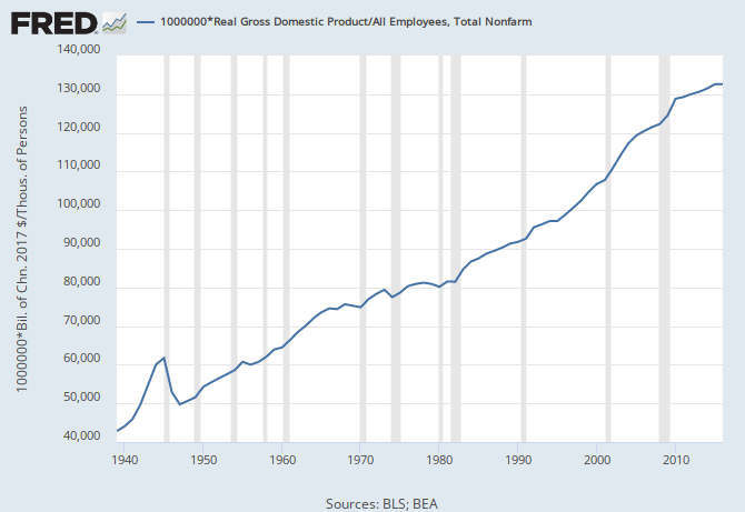
Real output per worker, 1921-1939:

The Depression didn’t just see a fall in employment, it saw a fall in the output of those still employed, reversing much of the productivity gains of the 1920s. (This surprised Keynes, among others, who still believed in the declining marginal product of labor, which predicted the opposite.) Recovery in the late 1930s, conversely, didn’t just mean higher employment, it involved a sharp acceleration in labor productivity. There’s a widespread idea that output per worker necessarily reflects supply-side factors — technology, skills, etc. But if demand had such direct effects on labor productivity in the Great Depression, why not in the Lesser Depression too? But for some reason, people who scoff at the idea of the “Great Forgetting” of the 1930s have no trouble believing that the drastic slowdown in productivity growth of recent years has nothing to do with the economic crisis it immediately followed.

EDIT: I should add: While the decline in production during the Depression was, of course, primarily a matter of reduced employment, the decline in productivity was not trivial. If output per employee had continued to rise in the first half of the 1930s at the same rate as in 1920s, the total fall in output would have been on the order of 25 percent rather than 33 percent.

Note also that the only other comparable (in fact larger) fall in GDP per worker came in the immediate postwar demobilization period 1945-1947. I’ve never understood the current convention that says we should ignore the depression and wartime experience when thinking about macroeconomic relationships. Previous generations thought just the opposite — that we can learn the most about how the system operates from these kinds of extreme events, that “the prime test of Keynesian theory must be the Great Depression.” Isn’t it logical, if you want to understand how shifts in aggregate demand affect economic outcomes, that you would look first at the biggest such shifts, where the effects should be clearest? The impact of these two big demand shifts on output per worker, seem like good reason to expect such effects in general.

And it’s not hard to explain why. In real economies, there are great disparities in the value of the labor performed by similar people, and immense excess capacity in the form of low-productivity jobs accepted for lack of anything better. Increased demand mobilizes that capacity. When the munitions factories are running full tilt, no one works shining shoes.

Plausibility

This shows the initial deviation of real per-capita GDP from its long run trend, and the average growth rate over the following ten years, for 1925 through 2005. The long run trend is based on the 1925-2005 average growth rate of real per-capita GDP of 2.3%. The points in the upper left are the ten-year periods beginning in 1931 through 1941.

UPDATE: A number of people have objected to this exercise on the grounds that the Depression and World War II period is not relevant for our current situation. I don’t agree with this. But even without them, the picture is not so different. While the postwar period up til now has never seen a persistent deviation from trend as we are experiencing now, or as rapid growth as the Friedman paper projects, the relationship between the two is clearly present. And a decade of growth far above the postwar norm turns out to be just what you would predict on the basis of that relationship. Here’s the same graph as above, but this time using only 1947-2005.

As you can see, the relationship is a fairly strong one. The Friedman growth number does lie a bit above the regression line. But it’s still true that the current exceptionally low level of GDP relative to trend would, on historical evidence, lead us to expect that growth over the next ten years will be around 3.8 percent — well above anything previously seen in the postwar period and close to double the long-term average.

Note that the seven points well below the line in the middle are 1999-2005, whose 10-year growth windows include the Great Recession. Without them, Friedman’s number would be much closer to the line. What do we make of that? Should the exceptionally poor performance of this period make us more pessimistic about medium-term growth prospects (it’s sign of supply-side exhaustion) or more optimistic (it’s a sign of a demand gap that can be filled)? This is not an easy question to answer. But just counting up previous growth rates won’t help answer it.

Can Sanders Do It?

My old professor Jerry Friedman wrote a piece several weeks ago, arguing that a combination of increased public spending and income redistribution (higher minimum wages and other employment regulation favorable to labor) proposed by the Sanders campaign could substantially boost growth and employment during his presidency. As readers of this blog know, this piece has gotten a lot of attention in the past couple of days. Most notably, it inspired a letter from four former CEA chairs strongly rejecting the claim that Sanders proposals could “have huge beneficial impacts on growth rates, income and employment that exceed even the most grandiose predictions by Republicans about the impact of their tax cut proposals.” A number of prominent liberal economists have endorsed the CEA letter or expressed similar doubts.

I want to try to clarify the stakes in this debate. There are three questions, each logically prior to the other.

1. Is it reasonable to think that better macroeconomic policy could deliver substantially higher output and employment?
2. Are the kinds of things proposed by Sanders capable in principle of getting us there?
3. Are the specific numbers in Sanders’ proposals the right ones for such a really-full employment plan?

The second question doesn’t matter until we’ve answered yes to the first one. And the third doesn’t matter until we’ve answered yes to the first two.

The first question is not only logically prior, it also seems to be what the public debate is actually about . The CEA letter, and almost all the other criticism of the Friedman paper I have seen, focuses on whether the outcomes described are plausible at all, not the specific ways they are derived from the Sanders proposals. Almost all the pushback I have seen has been to the effect that 5 percent real GDP growth and 275,000 new jobs per month are not possible results of any conceivable macro policies.

As I’m sure Jerry Friedman would agree, there are plenty of ways his estimates could be improved. But it’s pointless, even disingenuous, to debate the specific numbers before agreeing on the larger questions. I want to focus on the first question here, both because it is the premise of the others and because it is where the debate is currently located.

So: Is it plausible that there could be 5 percent-plus real GDP growth and 300,000 new jobs per month over the eight years of a Sanders presidency? I think it is — or at least, I don’t think there is a good economic argument that it’s not.

I want to make five related points here. First, conventional wisdom in economics is that an exceptionally deep recession should be followed by a period of exceptionally strong growth. Second, the growth in output and employment implied by the paper are more or less what is required to return to the pre-recession trend. Third, discussions of macroeconomic policy in other contexts imply the possibility of growth qualitatively similar to what Jerry describes. Fourth, it is not necessarily the case that the employment Jerry projects would exceed full employment in any meaningful sense. Fifth, if you don’t believe a growth performance at this level is possible, that implies a sharp slowdown in potential output, for which you need a credible story. The last point is probably the most important.
1. It’s not controversial to say that a historically deep recession ought to be followed by a period of historically strong growth. Every macroeconomics textbook teaches that changes in GDP can be split into two components: short-run variation driven by aggregate demand and by monetary and financial factors, and a long-run trend driven by population growth and technological change. While all sorts of things that constrain or inhibit spending can cause temporary dips in production, over time it should converge back to the fundamentals-determined trend. Unless they involve the destruction of real resources — and they don’t — recessions should not have lasting effects. A direct corollary of this textbook view is that the deeper the recession, the stronger should be growth in the following period — otherwise, there’s no way to get back to trend. The people who are saying that Jerry’s growth numbers are impossible on their face are implicitly saying that that we should expect all output losses in recessions to be permanent. This is not orthodox economic theory, at all. Orthodoxy says that the exceptionally deep recession should be followed by a period of exceptionally strong growth — and if it hasn’t been, that suggests some ongoing demand problem which policy can reasonably be expected to solve.
2. Friedman’s growth estimates are just what you need to get output and employment back to trend. This point is well made by Matthew Klein. As Klein puts it, this “supposedly ‘extreme’ and ‘unsupportable’ forecast implies American output will return to its previous trend just as Sanders would be finishing up his second term, in the third quarter of 2024.”

As Klein and others point out, the level of GDP projected by Jerry for the end of Sanders’ second term is right in line with what the CBO and other establishment forecasters were saying just a few years ago. I just now was looking at the CBO’s forecasts as of January 2013; they were projecting 4-4.5 percent real GDP growth over 2016-2017. This is, of course, exceptionally high by historical standards — Paul Krugman says that Jeb Bush was “rightly mocked” by progressives for suggesting he could deliver growth at that level. But the CBO was making the same prediction and it’s no mystery why — a period of growth well above historical levels is the logical condition of a return of output to trend. By the way, I should emphasize that Friedman’s growth estimates were not derived this way. It’s just a lucky coincidence — if it holds up — that the measures proposed by the Sanders campaign happen to be the right magnitude to close the output gap over eight years.

Similarly, Friedman’s employment numbers (around 277,000 new jobs per month) are indeed way above what we have seen recently. But if you want to get the employment-population ratio back to its 2006 levels by 2024, you need even more than that — about 300,000 new jobs per month, by my calculations. Many respectable economists — including at least one of the CEA signers — have written that the employment ratio is a better indicator of labor-market conditions than the unemployment rate, and expressed concern about its decline. A few years ago, Brad DeLong had no doubt that more expansionary policy could raise the employment population ratio back to 60.8 percent, if not to the pre-recession level of 63 percent: “we could still put 5.5 million more people to work with appropriate demand-management policies.” To do that by 2024 would imply monthly job growth around 220,000 — less than what Friedman claims for the Sanders proposals, but ~~about double what~~ ~~we are seeing now~~ more than double what the CBO is currently projecting for 2017-2024. It’s just arithmetic: you can’t raise the employment-population ratio without a sustained period of job growth substantially higher than what we are seeing now. So it makes no sense to talk about that as a goal if you think that faster job growth is not a feasible outcome for policy.

It is true, of course, that the aging of the population implies a long-term fall in the employment ratio, all else equal. But let’s put this in perspective. DeLong, for example, suggests that 0.13 points per year is probably an overestimate of the decline due to demographics. David Rosnick, applying the 2006 employment ratios of various age groups to the population projected for 2026, finds a larger decline due to demographics, on the order of 0.25 points per year. But even that leaves most of the fall in employment unexplained by demographics. By any standard, there is a lot of room to do better. But we have to agree that this is something that, in principle, demand side policy can do.

rosnick-2014-12-23-fig4 — *from David Rosnick*

3. In other contexts, it’s taken for granted that more expansionary policy could deliver substantially higher growth. Anyone who says that the zero lower bound is a constraint on monetary policy, or who suggests that the “natural rate of interest” is negative, is saying that output could be substantially higher given more expansionary monetary policy. Presumably, this is true for other forms of expansionary policy as well. (In terms of the model beloved by undergraduate textbooks and New York Times columnists: If the preferred point in ISLM space is to the right of the current one, we should be able to get there by shifting the IS curve just as well as by shifting the LM curve.) Obviously, the transition to that higher level of GDP would involve a period of much higher growth. It would be interesting to ask how fast output would have grown if we’d been able to remove the ZLB constraint in, say, 2010; I suspect the numbers might not look that different from Friedman’s.

Similarly, most participants in this debate agree that the ARRA stimulus of 2009 was effective, with multipliers above 2.0 for at least some categories of spending. Many also think that it should have been bigger. If increased government spending could boost output in 2008, then why couldn’t it today? And if the right answer to “how big?” then was “enough to close the output gap,” why isn’t that the right answer today? Yes, it would be a big number. (Again, it’s a lucky coincidence — if correct — that it happens to be close to what Sanders is proposing.) But so what? If “a trillion has a lot of zeroes” wasn’t a good argument against an adequate stimulus in 2009, then it isn’t one today.

Or again: If we think that austerity explains a big part of poor growth in European countries, we have to at least consider the the same might be true here. It would be very good luck, to say the least, if years of feuding between the administration and Republican congresses had somehow delivered exactly the right fiscal balance. In general, this discussion has been muddied by the fact that the pragmatic choice to delegate demand management to central banks, has been turned into an axiom in economic theory. From where I’m sitting, the statement “it would be helpful if the central bank set a lower interest rate” is equivalent, for most macroeconomic purposes, with the statement “it would be helpful if the level of public spending were higher.”

4. Friedman’s projections are unreasonable only if you think the US is already at full employment. The unstated but central premise of the critics is that we are at or near full employment, so there is no space for further demand policy. Friedman’s paper says that by the end of a second Sanders term, unemployment would be at 3.8%. Krugman replies: “It’s possible that we can get unemployment down under 4 percent, but that’s way below any estimates I’ve seen of the level of unemployment consistent with moderate inflation.” Now here we have an interesting question. Whether we are at full employment today depends, first, on how much you think the fall in the employment-population ratio reflects weak demand as opposed to structural or demographic factors — or in other words, to what extent faster job growth would draw nonworkers into the labor market, as opposed to pushing down the unemployment rate. But it also depends on what you think full employment means.

If you believe that any demand-induced acceleration of nominal wage growth will be passed to higher prices, or if you think that price stability should be the sole concern of macro policy, then there will be a hard floor on unemployment, which may not be much lower than where we are today. But if you think some appreciable fraction of faster nominal wage growth would go to an increase in the wage share (or faster productivity growth) rather than to inflation, and if you think some acceleration in inflation is acceptable (or even desirable), then “full employment” becomes a broad region rather than a sharp line. (I wrote a bit about these issues here.) In this case there will even be an argument — made by plenty of mainstream people, including some of the ones criticizing Friedman now — that a period of “overfull” employment would be desirable to bring the wage share back up from its current historically low levels. To believe that a 3.8% unemployment rate is ruled out by price stability considerations is to claim that faster wage growth cannot raise the wage share, which I don’t think is well supported either theoretically or empirically. (Or that raising the wage share is not desirable.) Also worth recalling: In the debates around the NAIRU in the 1990s, the general conclusion was that the idea of a hard floor to unemployment below which inflation will rise uncontrollably, is not in fact a useful guide for policy.

5. The argument against Friedman’s piece comes down to the claim that the economy is already close to potential. If this is the case then, yes, claims that increased public spending can achieve large gains in output are delusional. I think this is a useful debate to have, but I’m not sure how the CEA chairs would make the case. First, again, many of those criticizing Friedman’s numbers have supported the idea of more expansionary policy in other contexts. Second and more fundamentally, the persistent fall in the employment population ratio and the deviation of output from pre-recession trend seem very hard to explain in “supply” terms. Yes, there are demographic changes, but again, even if you hold the age distribution of the population constant, the employment ratio is still 3 points lower than at the start of the recession. That’s a deficit of 10 million jobs. Closing that gap requires an extended period of above average growth, qualitatively similar to what Friedman describes. If you believe that’s impossible, you have to explain why.

Logically, there are a couple possible answers. Either you argue that the earlier estimates of potential GDP were exaggerated, and we were at overfull employment prior to the recession. If you take this route, you have to be ready to make the case that the country needed substantially slower growth and higher unemployment in the 2000s, despite the noticeable lack of wage growth or rising inflation. Or, you can claim that something happened in 2008-2009 that permanently reduced potential output. So then, what is the negative technological shock that hit the economy in 2008-2009? Is Casey Mulligan right that American businesses have been crippled by the red tape of Obamacare? I don’t think either of those are good options for liberals. Another possibility is to talk about hysteresis and so on — the persistent effects on the laborforce and productivity growth from periods of weak demand. Here you will be on firmer ground — there is plenty of evidence that deep recession inflict lasting harm on workers and businesses. But this kind of reasoning makes Friedman’s numbers more plausible, not less. Because if weak demand can drag potential output down, strong demand can presumably pull it up.

The bottom line is this. Ten years ago, the CBO expected GDP to be $20.5 trillion (correcting for inflation) as of the end of 2015. Today, it is $18.1, trillion, or about 12 percent lower. Similarly, the employment-population ratio fell by 5 points during the recession (from 63.4 to 58.4 percent) and has risen by only one point during the past six years of recovery. Either these facts — unprecedented in the postwar period — reflect a shortfall of effective demand, or they don’t. If they do reflect a lack of demand, then there is no reason the expanded pubic spending and downward redistribution that Sanders proposes cannot close the gap, with a period of high growth while output and employment return to trend. (The fact that such high growth hasn’t been seen in the postwar period is neither here nor there, since there also has been no comparable deviation from trend.) Alternatively, you may think that the shortfall relative to previous growth rates reflects a decline in potential output. But then you need to offer some explanation of why the growth of the economy’s productive capacity slowed so abruptly, and you need to apply this belief consistently. I think it’s more reasonable to believe that the gaps in output and employment reflect a demand shortfall. In which case, the Sanders plan could in principle have the kind of results Friedman describes.

UPDATE: There was a significant error in section 2, which I’ve corrected.

Wages, Productivity and Employment

In a previous post, I wrote:

Supporters of a higher minimum wage invoke efficiency wage arguments without explaining why that should be expected to dampen disemployment effects rather than amplify them. While opponents of higher minimum wages describe faster productivity growth as a cost, without, as far as I can tell, being against it in any other context. This is a case where abstraction — some equations, even one of those awful supply and demand graphs — might actually be helpful.

Well, for some reason, I sat down and did the math. And the results are interesting.

I need to stress at the outset: This is a “model,” in the sense that it is a set of mathematical equations that are intended to give a simplified description of a phenomenon in the real world. But it is not a model in the sense that you may be used to in economics. I am not making any behavioral assumptions here of any kind. I am simply trying to formalize the logical relationships that everyone in this conversation is discussing. For example, someone says “higher wages will increase labor productivity,” and someone else says, “no they won’t.” Then we can write

y = a w,

where y is the change in percentage output per worker, w is the percentage change in the wage, and a is a parameter. Writing it this way, and reframing the questions themes likely value of a, is not taking a position in the argument or adding anything to the statements that were made. It is just rephrasing them in a way that, first, allows for more precise statement of the disagreement (maybe both people actually agree that a is probably around 0.1, but one of them considers that a meaningful effect and the other thinks it is trivial) and, second, makes it possible to systematically explore how these claims are logically related to others. As soon as you have more than one or two quantitative relationships to fit together, it is easier to work with algebra than with words.

So let’s do it.

As in that other post, we will use lower case variables here as rates of change. e is the percentage change in employment, w is the percentage change in the wage, y is the percentage change in output per worker, q is the percentage change in the quantity of output, and p is the percentage change in the price of output. q and p apply to whatever firm, industry or region wages are increasing for. w, e and y are for whatever group of workers we are interested in — it doesn’t matter for this purpose whether we think of a minimum wage increase as a big percentage increase for a small group of workers (those directly affected) or a small percentage increase for a bigger group. a1 through a4 are parameters. I am writing as if the relationships are all linear, to keep things simpler. But I’m pretty sure everything would turn out the same with a more general functional form.

First, we know that employment depends on the quantity of goods produced and the amount of labor used for each one. So we can write [1]

(1) e = q – y

This is an accounting identity.

(2) q = – a1 p + a2 (e + w – p)

a1 here is the price elasticity of demand faced by the unit where wages have increased. a2 reflects the demand created by the wage increase; it is equivalent to the fraction of wages from the unit (firm, industry, region, etc.) in which wages are changing, that is spent on the output of that unit. We know a1 > 0, and a2 >= 0. For an individual business, or a relatively narrow group of businesses or workers (such as in the case of a minimum wage increase), a2 will be very low — McDonald’s employees are probably McDonald’s customers, yes, but the percent of their total income they spend there can’t be above single digits. Conversely, as we talk about a broader and broader wage increase, a1 will approach zero as there is less and less margin for substitution away from higher-cost producers. Probably there aren’t many cases where we need both parameters.

(3) p = a3 (w – y)

a3 is the fraction of changes in unit labor costs that are passed on to prices. We know that 0 <= a3 <= 1, with a3 = 1 describing a constant markup.

(4) y = a4 w

a4 is the fraction of (exogenous) wage increases that are absorbed in higher labor productivity. Assuming rational (profit-maximizing) behavior by businesses, 0 < a4 < 1 for wage increases imposed from outside. (For voluntary wage increases like the one depicted in the Doonesbury cartoon, presumably the employer thinks a4 > 1.) It doesn’t matter whether we imagine the substantive reality described by Equation 4 as an efficiency wage/motivation/turnover story, or a mechanization/robots story. [2] The question we are interested in is, what are the implications of a high value for a4 for the disemployment effects of an increase in wages?

First we combine these equations and express e as a function of w:

(5) e = w [ a3 (-a1 – a2) (1 – a4) + a2 – a4] / (1- a2)

This isn’t very transparent. For a simpler case, assume that the markup is fixed and demand effects are not important. So a3 = 1 (fixed markup) and a2 = 0 (no demand effects.). Then we have:

(6) e = w (-a1 + a1 a4 – a4)

It’s clearer here that the wages-productivity link enters twice. Which makes sense if you think about it. Higher productivity may translate into lower prices, which in turn may translate into higher sales. That’s the middle term, which also depends on the price elasticity of output. But on the other hand, higher productivity means lower employment per good produced. That’s the second term, –a4 by itself.

Which dominates? The answer is straightforward: For it to be the case that when higher wages lead to higher productivity, that ameliorates any employment loss from higher wages, it must be the case that the price elasticity of demand for goods is greater than one. But in this case, as you can see from equation (6), the employment elasticity with respect to the wage must be at least negative one — a one percent increase in wages must lead to at least a one percent fall in employment. Because in the best case, if wage increases are entirely offset by productivity improvements, then a4 = 1. In which case, we have e = w(-a1 + a1 – 1) = -w. (Recall that all variables here are in percent changes.)

So the conclusion is: if we assume a fixed markup and ignore the demand created by higher wages, it is impossible that efficiency-wage or other productivity stories can explain an absence of disemployment from minimum wage increases. If there are large disemployment effects, efficiency-wage type stories can explain why they are not even larger. But they cannot explain why we don’t see disemployment at all, if that is the case. This might seem like a strong conclusion but it really is unavoidable — and it’s actually quite logical when you think about it. Productivity gains only ameliorate the disemployment effects by moderating the reduction in sales that would otherwise result from higher prices. But they also reduce the number of workers required at any given level sales. The first effect can only dominate when the loss of sales is large, i.e. where there is already a substantial disemployment effect.

Now what if we reintroduce variable profit margins and demand from workers?

Take the derivative of (5) with respect to w (which just gives you the rest of the right hand side) and then with respect to a4, and that tells you how the (dis)employment effect of wage increase varies with the extent to which that increase results in higher productivity. This is:

(7) d(de/dw)/d a4 = [a3(a1 + a2) – 1] / (1 – a2)

For productivity gains to ameliorate rather than exacerbate the disemployment effect, this must be greater than one. Since a2 will always be less than one —affected workers can’t spend more than all of their incremental wages at affected employers — we can ignore the denominator. So we need:

(8) a3(a1 + a2) > 1

Notice that this includes the simple case we considered before, with fixed margins and no important demand from affected workers. Then a3 =1 and a2 = 0 so condition(8) is just that demand for relevant output have price elasticity of at least unity.

In the more general case, we can see that, if demand from the affected workers is important, high productivity is more likely to ameliorate disemployment effects. We have to think carefully, in this case, about how large a2 might plausibly be. Even if we are imaging an across-the-board wage increase in a closed economy, not all of the incremental wages will be spent concurrently produced goods. And in any real-world case, there will also be increased imports, and reduced investment and consumption out of profits. If we are considering one business or a limited sector, a2 will certainly be close to zero. For an economy as a whole,it might be bigger — but it also might be negative. (This is the whole debate about wage-led versus profit-led demand.) Meanwhile, recall that a3 is the share of higher costs that is passed on to prices. (So 1 – a3 gives the fall in profit margins.) Notice that if a3 is small, condition 8 will not be satisfied. In other words, if higher wages come out of profits, then any resulting productivity increases will mean more disemployment, not less.

Again, this initially comes out of the algebra, but if you think about it it makes sense. If costs can’t be passed on to prices, then higher productivity just goes straight to the bottom line. And if costs are not passed on to prices, then lower costs can’t lead to higher sales. All they mean is fewer workers needed for the same output. You might think — I did think, until I worked through this — that “higher wages will mean higher productivity” and “higher wages just come out of profits” reinforce each other as two reasons not to worry about higher wages costing jobs. But actually they are contradictory. Higher productivity only mitigates job losses if higher wages do not come out of profits.

Again, I want to emphasize that this is not a model in the usual economics sense of starting some standard description of individual behavior and then tweaking the assumptions so as to produce the desired results. [3] Rather, I am simply stating the claims everyone in the debate agrees on, and then asking what their logical implications are. In particular, no one disputes that higher productivity both offsets the effect of higher wages on costs, and reduces the number of workers required to produce a given output. But that doesn’t mean they consistently take both effects into account when they consider the effects of a wage increase.

Tl; dr:

Higher productivity alone cannot explain why disemployment effects so small. By itself, higher productivity will only ameliorates job loss if a one percent wage increase causes a fall in employment of more than one percent; otherwise, productivity gains will make the job loss worse. If demand from the affected workers is important, then productivity gains can help even if the elasticity is smaller than negative one, but probably not too much smaller. And to the extent cost increases come out of profits rather than being passed through to prices, productivity gains will definitely make job loss worse. These seem like strong conclusions, but they follow logically from premises that are disputed by no one — that higher productivity means that the same output an be produced by few workers, that higher costs may be passed on wholly or impart to higher prices, and that higher prices may result in lower sales.

One specific lesson I take from this is that the observed lack of disemployment from minimum wages must be the result of higher prices and/or lower profit margins, not efficiency wage type effects. In fact, the lack of observed job loss suggests rather strongly that productivity does not rise with higher wages. An interesting question is why people are so attracted to stories where it does.

UPDATE: I should add — I’m not labor economist, I have only a superficial knowledge of this literature; I’m sure someone else has done exactly this exercise and reached the same conclusions. I don’t claim I’m adding anything anything new. I just did this because I was puzzled about myself, and wanted to know under what conditions higher productivity would moderate job losses from higher wages, and under what conditions it would make them worse. And now I do.

[1] Again, using the fact that percentage changes are approximately equal to log differences.

[2] I wanted to explicitly justify this statement but the post is too long already.

[3] In my experience, it’s basically impossible to talk about this kind of thing with a professional economist without them immediately wanting to reframe it as problems optimization under constraints, even if that’s irrelevant to the question at hand. In this case, for instance, if we want to know what the effects of the wage increase are on sales, ,it’s sufficient to know how much the higher wage is passed on to prices, and how strongly sales fall with higher prices. Both these parameters might well be the result of maximization of profits (or some other objective) but you don’t need to know anything about that to answer to question. With respect to employment, what matters is whether the whole cost increase is passed on topics, or some it, or none; the effect will be the exactly same whether or not that fraction is the result of an optimization process.

Reading the FT: The European Central Bank Is Not the Central Bank of Europe

A couple interesting pieces in yesterday’s Financial Times, related to last year’s debates about the role of the ECB in the European crisis.

First, this article on proposals to scrap higher-denomination bills (to combat money laundering) notes in passing that “the Central Bank of Luxembourg is a particularly prolific producer of high-denomination notes … Luxembourg issued notes equivalent to 194 percent of its GDP in 2013, compare with 16 percent in Germany, 9 percent in Italy and 4 percent in France.” This is a nice reminder that the printing of banknotes is not centralized in Europe, but — like almost all the day-to-day activity of central banking — remains the responsibility of the various central banks, with little oversight from the center. This little story is also a reminder of how — as I’ve pointed out before — the eurosystem is not like the gold standard. The exceptionally large cash issues in Luxembourg are an issue for law enforcement or financial regulators, but they are not a macroeconomic issue. No one suggests that large cash issues could ever cause the Bank of Luxembourg to exhaust its reserves, in the way that equivalent “internal drains” occasionally threatened the Bank of England in the 19th century. I wish in retrospect than I’d written something during the Greek crisis mentioning that physical euros are in fact already printed in Greece. Not that I think this operational detail is very important in itself, but it crystallizes the continued role, (and potential autonomy) of the national central banks in a way that more abstract arguments don’t.

Second, on the op-ed page there is Wolfgang Munchau suggesting that one of the main reasons for the revival of the German economy in the early years of Nazi rule was the accomodative policy followed by Hjalmar Schacht at the Reichbank, which included not only conventional expansionary policy — enabled by effective exit from the gold standard — but “unilateral restructuring of private debt owed by German companies to foreigners.” (Schacht’s memoir My First 76 Years is fascinating reading.) The recovery of output and employment in Germany ahead of the rest of Western Europe, Munchau writes, was “one reason for Hitler’s initial popularity,” and, more to the point, is evidence for “what an unorthodox central banker can do if he or she has the political support to break with the prevailing orthodoxy.” The relevance for today is obvious:

The current policy orthodoxy in Brussels and Frankfurt, which is shared across northern Europe, has some parallels to the deflationary mindset that prevailed in the 1930s. Today’s politicians and central bankers are fixated with fiscal targets and debt reduction. As in the early 1930s, policy orthodoxy has pathological qualities. Whenever they run out of things to say, today’s central bankers refer to “structural reforms”, although they never say what precisely such reforms would achieve.

In principle, the eurozone’s economic problems are not hard to solve: the European Central Bank could hand each citizen a cheque for €10,000. The inflation problem would be solved within days. Or the ECB could issue its own IOUs — which is what Schacht did. Or else the EU could issue debt and the ECB would buy it up. There are lots of ways to print money. They are all magnificent — and illegal.

There are no Nazi parties in the eurozone today, except in Greece. But France and Italy have populist parties on the right that are clearly outside the current policy consensus. Imagine a scenario in which Beppe Grillo, leader of Italy’s Five Star Movement, were to win the Italian election in 2018.

The term of Ignazio Visco, governor or the Bank of Italy, expires in November that year. Mr Grillo would be in a position to appoint his own central banker. Perhaps he would choose someone as resourceful and ruthless as Schacht and able to plot Italy’s way out of the euro, via a parallel currency regime for a transitional period, defaulting on foreign debt in the process. The devaluation and the increase in public sector investment which would be possible under a new regime could bring instant economic growth.

This is interesting, for a couple of reasons. First, the assumption, which Munchau doesn’t feel he needs to defend or even state explicitly, that any elected European government can appoint its own central bank leadership, without the approval of the ECB. (My understanding is that this is indeed the case, though the relevant national laws all include sweeping but presumably unenforceable language that once appointed the central bank leadership is not to take any outside direction.) Also worth noting, the suggestion of a temporary parallel currency, consistent with my idea that exit from the euro would not have to be an all-or-nothing leap, but involves passing through an extended gray area.

The second interesting thing is Munchau’s evident ambivalence. On the one hand, he sees the parallels between today’s the orthodoxy of the euro today and of the gold standard before World War II. [1] He recognizes the problems with postulating objective constraints on central banks in a depressed economy. He realizes that the current austerity regime shows no signs of delivering material benefits to the great majority of Europeans. And against this … what? “I have no doubt that any populist government in Europe would end in disaster,” he writes, but the basis of this certainty is not explained.

For myself, I have no doubt that the European crisis is not over. At some point, maybe soon, another European government is going to come up hard against the limits of acceptable policy in the Brussels-Frankfurt orthodoxy. I still think the national central banks will be the commanding heights in the ensuing battle.

[1] To be clear: I don’t think there is a close parallel in the way the two systems actually operate, but in their ideology, yes.

Minimum Wages: A Puzzle

Doonesbury

This, presumably, is a pro-minimum wage cartoon. This, clearly, is an anti-minimum wage column. But putting our economist’s hat on for a second — aren’t they making the same argument?

This has bugged me about the minimum wage debates for a while. Supporters say, mandating higher wages will lead to more motivated employees, less turnover and training costs, less need for supervision. Opponents say, mandating higher wages will lead to mechanization of jobs currently done by low-wage labor, substitution of capital for labor. But at an abstract level, it seems to me these are just two ways of describing the same thing. Aren’t they both just saying, faster growth of labor productivity? How can the same predicted outcome be an argument both for and against higher wages?

The anti- side seems to be implicitly assuming a fixed quantity of output, so that less labor per unit means less labor overall. The pro- side seems to be implicitly assuming some combination of a flat demand curve and a flattish supply curve, so that a fall in costs leads to a large rise in output. But you’ll still get some fall in employment, in the absence of monopsony or demand effects.

Anyway my interest here is not in what is the right answer. [1] My interest is that supporters of a higher minimum wage invoke efficiency wage arguments without explaining why that should be expected to dampen disemployment effects rather than amplify them. While opponents of higher minimum wages describe faster productivity growth as a cost, without, as far as I can tell, being against it in any other context. This is a case where abstraction — some equations, even one of those awful supply and demand graphs — might actually be helpful.

[1] Just to be clear, I support a higher minimum wage, $15, whatever. A few years ago, I even testified to that effect before the Maryland state legislature.